Enhancing 2D-LC Analysis using the Multiple Heart-Cutting Technology

This article describes the concept of multiple heart-cutting (MHC) 2D-LC, which advances heart-cutting analysis to a higher level. Innovative interfacing technology facilitates parking of 1D aliquots while running 2D cycles. In this way, heart-cuts can be taken from multiple 1D peaks at high frequency, which provides detailed information on target components. The technique is completed by specific 2D-LC software assisting in method setup and evaluation of MHC data.

1 Introduction
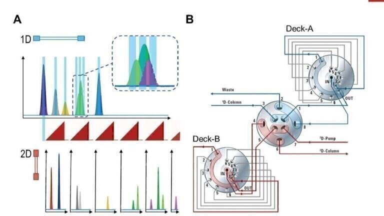
Two-dimensional liquid chromatography (2D-LC) has been demonstrated to greatly enhance separation performance compared to conventional 1D-LC and becomes applicable when samples are complex. In principle, a 2D-LC system consists of two single LC instruments that are interfaced via the 2D-injector as shown in Figure 1 (A). A 2D-LC experiment starts with 1D-chromatography. Aliquots of the effluent of the 1D-column are sampled and subsequently injected onto the 2D-column for further analysis. It is mostly the difference in selectivity that governs the separation. In the ideal scenario, where the separation mechanism in 1D is orthogonal to that in 2D, resolving powers (peak capacities) multiply [1,2].
In the past alternating dual loop interfaces have mostly been used [2]. Figure 1 (A) shows a 2-position/4-port Duo Valve that has two symmetric flow paths and has been developed specifically for its application in 2D-LC. On the basis of design, it minimises pressure fluctuations at the inlet of the 2D-column (that inevitably occur upon valve switching), which extends column life time substantially [3]. 2D-LC initiates in position-1 of the valve, where the 1D-effluent passes through loop-1 (blue path). The valve switch to position-2 injects the contents of loop-1 into the 2D-cycle. Once this 2D-separation has finished, the sample in loop-2 can be injected. The process is then repeated as necessary.
2D-LC can be divided into two major types of operation, comprehensive and heart-cutting. The application of each mode depends on the task.
The task for comprehensive 2D-LC is typically to gather all information possible from unknowns of high complexity such as found in Omic-type applications, natural products, and the analysis of biomolecules [e.g. 4]. Accordingly, all the material eluting from the 1D-column (regularly the entire 1D-effluent) is sampled and transferred to 2D. Sampling should occur frequently to avoid re-mixing of components that had been successfully separated in 1D [5]. These conditions entail a typical 2D-LC operation with swift gradients, short columns, and high flow rates in 2D and reduced flows in 1D because the duration of the 2D-cycle is normally equivalent to that of sampling.
The purpose of heart-cutting 2D-LC is quite different from that of comprehensive chromatography in that it aims to determine only one or a few compounds, characteristically in samples of high complexity. As shown in Figure 1 (B), only a distinct fraction of the 1D-peak is taken for reanalysis in 2D. This breaks the link between sampling time and 2D-cycle so that both dimensions can operate at more optimal conditions allowing for use of longer gradients and columns with higher separation efficiency in 2D, which often leads to improved chromatography compared to comprehensive mode. Further there is no absolute need to reduce flow rates in 1D [6]. Such win of chromatographic quality comes at a price, which in this case is the potential loss of information. For instance, the schematic in Figure 1 (B) points out the omission of grey, orange, and blue 1D-peaks during 2D-cycles of cut #1 and 2, respectively. The inset shows that there might be more underneath the green peak.

Multiple Heart-Cutting (MHC) 2D-LC
This article describes multiple heart-cutting (MHC) 2D-LC, a technique that antagonises loss of relevant information in that it permits parking of additional cuts while running the 2D-cycle. This is illustrated in Figure 2 (A). Heart-cuts are taken from multiple 1D-peaks and a more frequent sampling allows for the detailed examination specifically of the green peak.
The parking concept is supported by new interface technology. One configuration is shown in the diagram of Figure 2 (B). Sampling loops of the dual loop interface are replaced by ‘(parking) decks’, each bearing six loops. Thus, this MHC interface offers twelve sampling positions.
MHC 2D-LC example applications will demonstrate:
• 2D-LC software that markedly facilitates MHC method setup and data evaluation.
• The routine for detailed determination of multiple target compounds.
• Features to ensure repeatability and correctness of results.
• MHC 2D-LC quantification performance.   

2 Method Setup and Experimental
Data were acquired using the Agilent 1290 Infinity 2D-LC Solution with Multiple Heart-Cutting that was operated using OpenLAB CDS ChemStation Edition C.01.07 extended by 2D-LC package.
Samples were dilutions of the Agilent 2D-LC starter sample. It contains 16 small molecular weight compounds, each at a concentration of 1 mg/mL: atrazine, chlorotoluron, desethylatrazine, desethylterbuthylazine, diuron, hexazinone, linuron, metazachlor, methabenzthiazuron, metobromuron, metoxuron, nifedipine, nimodipine, prometryn, sebuthylazine, and terbuthylazine. Dilutions were prepared freshly before analysis in 1D mobile phase (A/B 80:20 v/v).
 
2.1 First dimension (1D)
1D used either 1290 Infinity Quaternary or 1290 Binary Pump, Autosampler, Thermostatted Column Compartment (TCC) and DAD detector with 10 mm flow cell tracking the 254 nm trace. Column was of the type Zorbax SB C18 100 x 2.1 mm 1.8 µm held at 40°C. Mobile phase A was 0.2% formic acid (FA) in water and B was methanol. Gradients went from 20 to 100 %B in 50 minutes at a flow rate of 600 µL/min.

2.2 Second dimension (2D)
2D used a 1290 Infinity Binary Pump. Column was Zorbax Bonus RP (50 x 2.1 mm, 1.8 µm) held at 40°C. Bonus RP (a polar embedded amine column) has been demonstrated to provide markedly different selectivity than SB C18 for polar compounds [6]. The DAD detector was equipped with 10 mm or 60 mm max light cartridge cells acquiring at 254 nm.
All experiments used the MHC 2D-LC interface as shown in Figure 2 (B). In detail, 6-pos/14-port selector valves are connected to the 2-pos/4-port Duo Valve. Each selector bears a cluster of 6 preinstalled 40 µL sampling loops. This provides two parking decks (A and B) with 12 loop positions in total. The switch of the Duo Valve places a deck in sampling or alternatively in 2D-analysis position. The switch of the selector valves provides access to the discrete loop positions.
Mobile phase A was 0.2% FA and B was acetonitrile. Data were acquired using a 2D cycle time of 1.75 minutes. A flow of 1 mL/min was used. Initial gradient was from 10 to 60 %B in 1.25 minutes. A gradient shift was programmed to reach a start condition of 30 %B at 20 minutes. The described 2D-specific settings are organised in the method setup dialog shown in Figure 3. Panels: 2D-LC mode (A), solvents (B), flow settings (C), 2D-gradient (D), 2D time segments (E), operating values (F), gradient preview (G), and zoom out of the 2D-gradient at initial condition (H). A more detailed description extends the scope of this article and can be found in the instrument user guide [8].
3 Software features and operational routine
3.1 Gradient preview
The preview displays the 1D gradient (red trace) and predicted 2D-cycles superimposed (blue trace) as shown in Figure 3 (G). A 2D-gradient shift can be edited using this graphical interface by reference point values, which can be mouse-dragged to the desired location. Preview and tables (D and E) are interconnected so that any graphical change is automatically reflected in the tables and vice-versa. A 1D UV-chromatogram (black trace) can be uploaded, which can be from any previously acquired run. In this case the chromatogram was obtained from a 2µL injection of a 1:10 dilution of the 2D-LC sample.
Multiple heart-cutting experiments can be performed in two operational modes, peak based and time based. In peak based mode, heart-cuts will automatically be taken for 2D-analyses upon 1D-peak recognition. The system is activated for sampling when a peak is sensed by the 1D-detector. The trigger for this can be a baseline threshold, slope, or the combination of both. Sampling stops when the trigger matches a second time (indicating the end of the peak), or alternatively when the sampling time (set in segment (E) of Figure 3) has elapsed. The software accounts for the (peak) transport delay between 1D-peak detection (peak located in the UV flow cell) and its arrival at sampling loop inlet.
Figure 4 shows detailed views of gradient previews. These experiments used a baseline threshold (50 mAU) for peak detection and sampling time was set to 1 minute, which exceeded the peak width by far so that solely the 1D-detector signal ruled sampling. The green coloration is indicative for the peak based mode and predicts the trigger interval for this uploaded chromatogram. Panel (A) shows the preview obtained with the MHC interface and panel (B) the case if a dual loop interface were used. The software shows red marks for heart-cuts that cannot be made.   
In time based mode, sampling is triggered by time events as specified by the operator. The software assists in that it automatically generates a heart-cut timetable (Figure 3 (E)) based on the uploaded chromatogram using criteria as in peak based mode. The corresponding orange markings in the preview (Figure 3 (G)) designate the heart-cuts that will be made in this experiment.

3.2 Sampling/parking algorithm
The MHC algorithm reduces valve switches to a minimum but follows the rule to promptly process heart-cuts that are sampled or parked.
The first heart-cut is always sampled in loop-1 of deck-A, and promptly submitted to its 2D-cycle. As long as the time difference between consecutive cuts exceeds the 2D cycle time, there is no parking required and the MHC interface works just like a dual loop interface sampling in loop-1 of each deck. That is only the Duo Valve operates, the decks do not switch. In the analysis in Figure 3, this would be the case for cuts #1 to 4.
Figure 5 (A) shows an excerpt of the 1D-chromatogram in Figure 3 representing 1D-regions in which parking occurs. Under current experimental conditions (1D-flow = 600 µL/min, loop size = 40 µL, sampling time = 0.13 min), the system was operated to overfill the loops twice as indicated by the trigger interval (orange markings). The shaded zone relates to the loop volume and is subsequently about half as wide as are the orange marks. It predicts more exactly which portion of the peak will be taken. Graphics (B) and (C) show snapshots of the 2D-LC online monitor. This is a part of the 2D-LC software, which traces the actual state of the sampling interface during the 2D-LC experiment. MHC decks are displayed schematically, each with six slots representing the sampling loops. In these slots cut numbers and the time of parking are displayed. Here, for reasons of illustration only cut numbers are shown.  
Figure 5 (B) reflects the situation corresponding to the point of ca. 14 min. During the 2D-run of cut #4 (loop-1, deck-B), cuts #5 to 9 were parked in deck-A (loops-1 to 5). Awaiting the processing of these cuts, deck-A remains connected to the first dimension (blue path) and therefore is set to a flow through position. The idle loop is always the loop one count greater than that where the last cut was parked. In the current case this is loop-6.
Monitor (C) shows the situation where the Duo Valve switched deck-A into 2D-analysis position currently processing cut #5 that was previously parked in loop-1. Deck-B connected to 1D has parked cuts #10 to 13 and waits in position-5 until deck-A has been completely analysed. After deck-B is switched back into 2D-position, deck-A once again offers its slots to 1D for sampling.   
While the parking process begins in loop-1 of a deck and succeeds in loops with increasing number, submission to 2D-analyses occurs in the reversed order. This has marked advantages but requires intuitive data analysis tools.

3.3 Data analysis
MHC data evaluation is assisted by the 2D-LC Heart-Cut Viewer. Figure 6 shows results obtained from the time based MHC experiment. The viewer displays the 1D-chromatogram (A), heart-cut table with sampling / parking details (B), the complete output of 2D (C), and an extracted view in panel (D). All panels are cross-linked to facilitate the process of data viewing. The shades with cut number support the match of cut and 2D-run. Blue highlights (panels (A - C)) indicate that heart-cuts #6 to 9 were selected. Corresponding 2D-results are superimposed in panel (D), which shows that three well separated peaks were obtained in contrast to the 1D-region sampled. Yellow marks with description ‘F’ represent a flush cycle, which is implemented to clean idle loop and connection capillaries between deck and duo valve.

4. Targeted Quantification
4.1 System linearity and sensitivity
Linearity experiments used dilutions of the 2D-LC starter sample in the range 0.5 to 1000 µg/mL, of which 2-µL volumes were injected at least in duplicate. Two 1D-regions were sampled, which is shown in Figure 7 (A) with the intention to quantify C1 and C2 co-eluting in region-1 and accordingly C7 and C8, which also partially co-elute with C6 in region-2. The MHC-interface was operated in partial loop fill mode with a sampling time of 0.06 min / cut (= 90% loop filling at used 1D-conditions) using time based sampling.
Figure 7 (B) shows 2D-chromatograms of cut #3 and 4 of region-1 and accordingly cut #7 and 9 of region-2 acquired at the lowest 0.5 µg/mL level. Prominent peaks were obtained in 2D. These were all well separated, which allowed for the integration of the single components. The peak heights exceeded those in 1D, despite heart-cutting. For instance, the 1D-peak (C1+C2) of which cut #4 was taken has a peak height of about 1 mAU. The corresponding 2D-run divided the signal into two peaks (C1 and C2) with heights of 3 and 4.5 mAU, respectively. The reason for this increased absorption was associated to the use of a 60 mm UV cell in the 2D detector. Different gradient slopes, solvents and type of detector could have played a role, too.
Figure 7 (C) shows log-plots of peak area versus concentration. The logarithmic scale better exhibits the linearity at the lower end. The top chart is from 1D-results obtained when integrating the peak (C1+C2) of region-1. It shows linearity across the entire concentration range investigated with a R2-value > 0.999. The chart on the bottom is representative for 2D-results and was generated from cycles of cut #4 (of region-1) and cut #9 (of region-2). Calibration plots, normalised to the area of the largest peak, are superimposed. The two highest levels exceeded the linear range of the detector but good linearity was measured down to 0.5 µg/mL with R2 > 0.999 for all four compounds (C1, C2, C7 and C8). System linearity and sensitivity of 2D as demonstrated here are important criteria for quantitation experiments as well as repeatability.

4.2 Repeatability
The repeatability of the 2D-analysis was determined from twenty consecutive 1µL injections of a 1:10 dilution of the 2D-LC starter sample. Figure 8 (A) shows 1D-chromatograms with cutting scheme and panel (B) 2D-chromatograms of cuts #5 to 9 overlaid (n=20).
The separation again was in all cases superior in 2D and the improved sensitivity, compared with 1D, agrees with findings reported above. Cut #5 to 9 comprised five components marked in Figure 8 as C1 to C5. Table-1 gives precision data (%RSD) calculated for peak areas, which normally were well below 10 %. Component C4 in cut #6 showed a few outliers. Close inspection revealed that when the area value in cut #6 was low it was higher in cut #7 and #8. It was difficult to tie this to any particular reason, but similar findings were made in the determination of additives in polymers, where even a very small retention shift in 1D caused an area variation [9]. This can occur because cuts are often made at the flank of the peak. One way to compensate for this is to sum peak areas of each component across the multiple cuts to give the total area. For example, the first injection in the current experiment gave areas for C4 of 420, 794 and 53 mAU*s, respectively in cut #6, 7, and 8 resulting in a total area of 1267 mAU*s. Table-1 demonstrates that RSD-values generally improved when using the total 2D-peak area for calculation with 1.6 %, 0.5% and 2.2 % for components C3, C4 and C5, respectively.