Understanding When Bigger is Best

It has been a notable trend for chromatographers to use smaller and smaller particles to drive the performance of their separation, however there are problems associated with this approach that mean on occasion bigger particles are actually better. Since the publication of the van Deemter equation it has been noted that there is an inverse relationship between the particle size and the chromatographic efficiency of a HPLC column. This has led to a gradual reduction in the particle size for the more leading-edge separations, with the bead technology being reduced from 10 μm down to the current state of play which is less than 2 μm. This has also led to the development of ultra-high pressure pumps to accommodate the increased pressure requirements associated with the smaller particles. Thus, the maximum operating pressures for commercially available chromatographic systems have seen an increase from 400 bar to over 1500 bar in the last two decades.

This would then suggest that for chromatographers the use of smaller particles is highly beneficial and that in all cases the smaller variant of particles should be used, however this is not the case but to better understand this statement it is necessary to better understand how chromatographic performance is measured. The most common approach to measuring chromatographic performance is to measure the efficiency and one measure of that is the use of experimental plates, which is obtained from the following equation.

Where;
tr is the retention time of the analyte, measured typically from the highest point of the peak response
w is the peak width at the base of the peak
In fact, what is being measured is the dispersion, or variance, of the analyte molecules within the chromatographic system. This dispersion is due to the random nature of movement of small molecules, and even though there is a general direction to the flow of the mobile phase, this random nature of dispersion will result in elements of the mobile phase moving at different linear velocities through the fluidic pathways.

Dispersion in the system

All molecules will have a degree of energy that can be utilised for movement within the space that they occupy. When looking at a large number of molecules there is a tendency for the molecules to preferentially move from areas of high concentration to areas of lower concentration. This can be summarised by Fick’s first and second laws of diffusion [1], relating to spatial and temporal concentration variations, which are given by;

These models do rely on a couple of assumptions though;
• The concentration of the solute is very dilute
• The solute molecules do not interact with each other
• There are no interactions with a container of any description
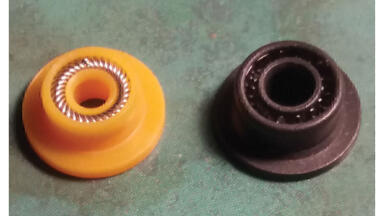
In a standard chromatography environment, the first of these two assumptions are valid. However, it is very evident that there will be a wall effect observed which will alter the effective dispersion processes within the tubing. Thus, it must be considered that when the diffusion in the mobile phase is contained in a fluidic pathway, the result will be in drag at the surfaces causing a parabolic flow profile across the tube, comparable to a bowl. Improving the radial movement of molecules will reduce this issue, as will reducing the diameter of the tubing, however for common connector dimensions the radial dispersion does not overcome the parabolic flow profile associated with the flow rates found in capillary HPLC. As a consequence of this effect increases in the flow rate will result in a greater variance, due to the frictional effects of the surface of the tubing being greater than the relative reduction in retention time within a capillary at the typical flow rates observed in capillary systems. This is typically measured by a parameter referred to as the variance.
The variance measures the amount of peak broadening and is the standard measure of how much dispersion there is within a chromatographic system. The smaller the variance, the less dispersion there will be. The degree of diffusion or dispersion has been effectively modelled by Aris and Taylor [2], resulting in this equation for a laminar flow system.

Where;
Deff is the effective dispersion coefficient
U is the average linear velocity
r is the internal radius of the connector
D is the measured dispersion coefficient
The important parameters to consider that will affect the dispersion rate are;

Viscosity of mobile phase

The mobile phase can have an effect on the dispersion processes, with the viscosity of the mobile phase being the most predominant parameter which will affect the dispersion. Thus, if a mobile phase is more viscous there is a tendency for the diffusion of the analyte to be less than that if the analyte were in a less viscous mobile phase. The change in the viscosity can be caused by a range of external effects, however the buffer concentration and also the temperature are the parameters which will have the greatest effect on the viscosity.

Diffusion coefficient of molecule

Another factor to consider is the diffusion of the molecule through the mobile phase. In this case the larger the molecule, in general, the greater will be the resistance to movement and so the diffusion coefficient will be lower.

Other Factors

The dispersion within the chromatographic system does not just come from the volume attributable to the volume of the tubing, but can also arise from the injection volume, the void volume of the column, the volume associated with an ill-fitting connector as well as the detector volume and can be summarised as;
V = Vinj + Vcol + Vtubing + Vconnectors + Vdetector cell
The volumes that each of these components contributes to the dispersion process within the chromatographic system can also be expressed in terms of a system variance with the individual variances having the same form as the above equation.
σ2total = σ2 inj + σ2 col + σ2 tubing + σ2 connectors + σ2 detector cell
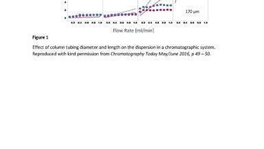
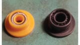
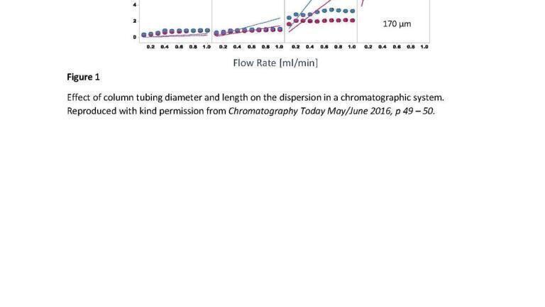
If the variance associated with the column is the major component of analyte retention time then changing the particle size to reduce this will have a beneficial effect, however if wider bore tubing is being used, or a large injection volume then the variance or dispersion associated with these components will dwarf the contribution from the column and thus changes in the particle size will not be detectable. The impact of using inappropriate connectors and tubing can be seen in Figure 1.

Kinetic Plots

However, this is not the only reason why smaller particles may not be beneficial and to get a better understanding for this interpretation it is necessary to look at the limitations of the initial modelling work associated with investigating dispersion within a column. The most notable work in this area was initially done by Jan Jozef van Deemter, a Dutch physicist working at the Royal Dutch Shell company as a researcher. His modelling work split the dispersion process into three key components, referred to as eddy dispersion (A term), longitudinal dispersion (B term) and dispersion associated with the resistance to mass transfer (C term) [3]. The model which bears his name has the form of;

Where;
HETP is the height equivalent to a theoretical plate, and is a measure of the peak width, smaller numbers are better.
u is the linear velocity of the mobile phase
A is the eddy diffusion constant, and is inversely related to particle size
B is the longitudinal diffusion
Cs and Cm are the diffusional constants of the analyte in the mobile phase and in the stationary phase, and is related to the particle size.
This work has been reviewed and updated on numerous occasions; however, the underlying structure of the equation has not altered. The above model does not take into consideration pressure and it does not consider time, both of the parameters are important from a practical perspective. In order to better understand these practical limitations, it is necessary to look at a different modeming approach, namely kinetic plots [4-10].
To perform the modelling three equations will be used.

Where;
N is the efficiency of the column defined by the equation.
L is the length of the column
u0 is the linear velocity of the mobile phase
t0 is time of a peak, in this case an unretained peak.
dp is the particle size
ΔPmax is the maximum operating pressure
Φ is the column resistance factor
η is the dynamic viscosity of the mobile phase
In the van Deemter plots HETP is plotted against the linear velocity u, with Figure 2 showing a plot of three different particle sizes, 1.8, 3.0 and 5.0 μm, with a clear benefit in smaller HETP values as the particles are reduced. On the right-hand side for Figure 2, shows a plot of log t0 versus log N. It uses the same data but also looks at the impact of column length and pressure in accordance with the three equations given previously. In these plots we will focus on the maximum log N that can be achieved.
The solid line represents the point of inflexion, or the point where the most efficient chromatography, sharpest peak relative to retention time, is obtained. As with the van Deemter plots the smaller particles clearly provide sharper peaks. The dashed line, however, represents where the column would be operating above the maximum operating pressure of the chromatographic system and so would not be obtainable in a practical sense. It can be clearly seen that for the smaller particles this has quite a significant effect on the performance capability when practical considerations are taken into account.
Taking the analysis further it is possible to plot the maximum practical performance of the column as shown in Figure 3. This plot is referred to as a constrained kinetic plot and takes into consideration real world parameters such as pressure. It can now be seen that the lines generated by the three different particle sizes cross, which then means that under different conditions different particle sizes should be considered to give the optimal performance. Thus the ability of a sub 2 μm to provide more chromatographic efficiency at increased analysis times is dramatically reduced, and that for longer analysis smaller particles will provide more chromatographic efficiency.
However, it could be said that the above work is all theoretical and so may not translate into a practical environment, however Figure 4 is based on experimental data and shows exactly the same trend as was seen with the theoretical data, demonstrating that bigger can truly be better for some forms of separations.

Conclusions

For many separation scientists today there is a tendency to focus on moving to smaller particles to drive separation performance, and the marketing hype associated with the use of small particles has been very intense. Indeed, the use of smaller particles can drive chromatographic performance under certain conditions, namely highly efficient separations performed in a short time performed on highly efficient chromatographic systems, the data provided in this article demonstrates this. It is not however, the panacea to solving separation scientists’ challenges, and having a thorough understanding of the theory can help ensure that the best operating conditions are chosen for a separation given the practical limitations of the instrumentation. As with most things we are far too often lured in with the headline figures and have our opinions swayed without really having a full understanding of all of the issues. Unfortunately, the world is not a simplistic place and having an ability to understand the nuances of an issue will hopefully ensure that we have a better understanding of what is happening but also ensure that we may make the correct choices.

References

1. Fick, A. Ann. der. Physik (in German) 94 (1855) 59
2. Aris, R., Proc. Roy. Soc. A., 235 (1956) 67–77
3. van Deemter J.J., Zuiderweg F.J. and Klinkenberg A., Chem. Eng. Sci., 5 (6): (1956) 271–289
4. Giddings, J.C., Anal. Chem. 37 (1965), 60-63
5. Knox, J.H. and Saleem, M.,J. Chromatogr. Sci. 7 (1969), 614-622
6. Knox, J.H., Annual Review of Physical Chemistry 24 (1973), 29-49
7. Guiochon, G., High-Performance Liquid Chromatography: Advances and Perspectives, Horvath,C., Ed.; Academic Press: New York, 1980; Vol. 2, pp 1-56
8. Hans, P., J. Chrom. A 778.1 (1997), 3-21
9. Desmet, G., Clicq, D. and Gzil, P., Anal. Chem. 77.13 (2005), 4058-4070
10. Carr, P.W., Wang, X., Anal. Chem. 2009, 81, 5342–5353